Reaction path search
Contents
Reaction path search#
For many computational studies the kinetics of a reaction are important to provide insights into the feasibility of reactions. Knowledge about the stationary points on the potential energy surface, like the minima and first order saddle points, provides the possibility to compute reaction energies as well as barrier heights. To obtain a path from the reactants to the products on the potential energy surface, different techniques have been proposed, here we will be focusing on the growing string method (GSM) to generate reaction paths.1
Setting up GSM#
For this tutorial we will use the GSM program available here.
While GSM has no native interface with DFTB+, it is possible to create an adapter which allows usage of DFTB+ from GSM.
The version of GSM used in this tutorial is gsm.orca, which is formally an interface to the Orca quantum chemistry program and will invoke a program called ograd.
Run script for DFTB+
Our adapter for DFTB+ is implementing such an ograd program as a simple shell script
#!/usr/bin/env bash
# SPDX-Identifier: Unlicense

# Break on errors and uninitialized variables
set -eu

# Get executables
dp2orca=$(which ${DP2ORCA:-dp2orca.awk})
dftbplus=$(which ${DFTBPLUS:-dftb+})

# All calculations are performed in scratch
if [ -f dftb_in.hsd ]; then
  cp dftb_in.hsd scratch/
fi
pushd scratch 2>&1 > /dev/null

# find the input files
input_file=$(realpath orcain$1.in)
output_file=$(realpath orcain$1.out)
geom_file=$(realpath structure$1)

# Prepare input file in xyz format
wc -l < "$geom_file" > struc.xyz
echo "Dummy" >> struc.xyz
cat "$geom_file" >> struc.xyz

# Run actual DFTB+ calculation
"$dftbplus" > dftb.out

# Post-processing, convert to Orca standard output
if [ -f results.tag ]; then
  "$dp2orca" results.tag > "$output_file"
fi
if [ -f autotest.tag ]; then
  "$dp2orca" autotest.tag > "$output_file"
fi

popd 2>&1 > /dev/null
Convert script gradient output
A companion script is provided to turn the DFTB+ produced nicely formatted output found in results.tag into the Orca standard output format
#!/usr/bin/awk -f
# SPDX-Identifier: Unlicense

# Produce expected output for GSM driver by writing Orca standard output.
END { orca_output(iat, mermin_energy, forces) }

# Write energy and gradient of the system in expected output format.
# This routine emulates the necessary parts of an Orca standard output.
#
# Input
# -----
#   nat: Number of atoms of the whole system
#   energy: Mermin free energy
#   forces: Atomic forces for each atom
#
# Output
# ------
#   Writes Orca formatted information to standard output
function orca_output(nat, energy, forces) {
  printf "ORCA-Dummy output for GSM TS Optimizer. Not a real ORCA-Output\n"
  printf "Total Energy       :  %20.14f\n", energy
  printf "------------------\n"
  printf "CARTESIAN GRADIENT\n"
  printf "------------------\n"
  printf "\n"
  for (jat = 1; jat <= nat; jat++) {
    printf "%4d%4s   :%15.9f%15.9f%15.9f\n", jat - 1, "X",
           -forces[jat][1], -forces[jat][2], -forces[jat][3]
  }
}

# Collect the energy and reset the flag.
read_energy > 0 {
  mermin_energy = $1
  read_energy--
}

# Collect a line from the force output.
read_forces > 0 {
  iat++
  for (ic = 1; ic <= NF; ic++) {
    forces[iat][ic] = $ic
    read_forces--
  }
}

# Label for total energy found.
/^mermin_energy/ { read_energy = 1 }

# Label for gradient found.
/^forces/ { gsub(/[:,]/, " ") }
/^forces/ {
  read_forces = 1
  for (dim = 1; dim <= $3; dim++) {
    read_forces *= $(3+dim)
  }
}
Make sure the ograd and dp2orca.awk script can be found in your executable PATH and are made executable.
With this setup we can run DFTB+ for computing our reaction path.
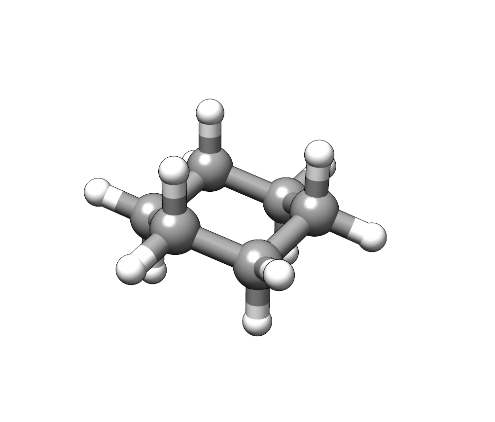
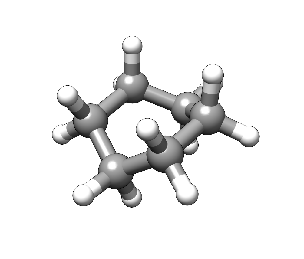
Cycloalkane inversion#
For our first application we will calculate the inversion barrier of a cyclohexane molecule. Create a new directory for this reaction and create the input file GSM. The most important settings are highlighted.
# FSM/GSM/SSM inpfileq
------------ String Info --------------------------------
SM_TYPE                 GSM    # SSM, FSM or GSM
RESTART                 0      # read restart.xyz
MAX_OPT_ITERS           80     # maximum iterations
STEP_OPT_ITERS          30     # for FSM/SSM
CONV_TOL                0.0005 # perp grad
ADD_NODE_TOL            0.1    # for GSM
SCALING                 1.0    # for opt steps
SSM_DQMAX               0.8    # add step size
GROWTH_DIRECTION        0      # normal/react/prod: 0/1/2
INT_THRESH              2.0    # intermediate detection
MIN_SPACING             5.0    # node spacing SSM
BOND_FRAGMENTS          1      # make IC's for fragments
INITIAL_OPT             0      # opt steps first node
FINAL_OPT               150    # opt steps last SSM node
PRODUCT_LIMIT           100.0  # kcal/mol
TS_FINAL_TYPE           0      # any/delta bond: 0/1
NNODES                  15     # including endpoints
---------------------------------------------------------
TS_FINAL_TYPE:Declares whether a bond is broken in the reaction.
0no bond breakage,1expect bond breakage.NNODES:Number of nodes in the reaction path. The number of nodes determines the computational cost of the reaction path search.
Next we need to provide the starting structures. For this purpose we use preoptimized structure of cyclohexane rotamers.
18

C         0.72407050811334    1.25235108200516   -0.24338094705465
C        -0.72343762657313    1.25319617766380    0.23929059852918
C        -1.44731174776017   -0.00012207898744   -0.24387881064420
C        -0.72448059275055   -1.25351379257321    0.24067027167326
C         0.72302665800789   -1.25441395902634   -0.24200633751896
C         1.44695184726671   -0.00106936630608    0.24102971332150
H         0.74079379322633    1.27977999101331   -1.33568337236737
H         1.23911262989111    2.14407418287692    0.12103331256485
H        -1.23773720847930    2.14497568327721   -0.12601425207736
H        -0.74014360366626    1.28171032471934    1.33155904823478
H        -2.47725186596728    0.00050340452584    0.12007291068245
H        -1.47894487592394   -0.00071222738449   -1.33620018565333
H        -0.74120355748858   -1.28080687484113    1.33297520098609
H        -1.23953398541620   -2.14527362819323   -0.12363941525185
H         1.23731965319244   -2.14616191699557    0.12338823394548
H         0.73972201150389   -1.28305135703018   -1.33427294070718
H         1.47879051289637   -0.00048052377193    1.33334318895494
H         2.47682744992731   -0.00169512097196   -0.12311621761763
18

C         0.73801367871811    1.26986541848913   -0.29891956390957
C        -0.72425034407001    1.23660126909089    0.13751131482082
C        -1.44534047314084   -0.03177648038732   -0.35671028842475
C        -0.51312926640361   -0.95386524177349   -1.13921033932034
C         0.73874270548611   -1.27320174695686   -0.32527750643084
C         1.46163460859193    0.00218599807452    0.14815613748902
H         0.80167461165837    1.37397900540374   -1.38290508569736
H         1.22823701649042    2.14109015941832    0.14110672721895
H        -1.22954714616749    2.12895335124983   -0.23651035666162
H        -0.75981821609326    1.27774751863575    1.22804091215143
H        -1.84194534594910   -0.58465393222957    0.49789315375467
H        -2.29332568018213    0.23757670740058   -0.98938629993452
H        -1.03732116020641   -1.88207230826469   -1.37787118249708
H        -0.23326413070136   -0.48637114937456   -2.08427188018927
H         0.44512664267991   -1.87161892139158    0.54024210888424
H         1.41101252131720   -1.88609677273023   -0.92920597460851
H         1.52271848431407    0.00555688995561    1.23838178865502
H         2.48432149365809    0.02132023538992   -0.23310366530028
For our first calculation we will use GFN2-xTB
Geometry = xyzFormat {
<<< "struc.xyz"
}

Hamiltonian = xTB {
  Method = "GFN2-xTB"
}

Options = {
  WriteAutotestTag = Yes
  WriteDetailedOut = No
}
Analysis { CalculateForces = Yes }
ParserOptions = { ParserVersion = 10 }
Parallel = { UseOmpThreads = Yes }
Prepare the computation by creating the initial string file in the scratch directory
❯ ln -s $(which ograd)
❯ mkdir scratch
❯ cat reactant.xyz product.xyz > scratch/initial0000.xyz
❯ tree .
.
├── dftb_in.hsd
├── inpfileq
├── ograd -> /path/to/ograd
├── product.xyz
├── reactant.xyz
└── scratch
    └── initial0000.xyz
Before we run the GSM calculation, we should make sure that our setup does work and all scripts are found correctly
❯ awk 'NR > 2 {print $0}' reactant.xyz > scratch/structure0000.test
❯ ./ograd 0000.test
❯ cat scratch/orcain0000.test.out
ORCA-Dummy output for GSM TS Optimizer. Not a real ORCA-Output
Total Energy       :    -18.98671575397980
------------------
CARTESIAN GRADIENT
------------------

   0   X   :   -0.000022175   -0.000032523    0.000045093
   1   X   :    0.000018687   -0.000029431   -0.000041726
   2   X   :    0.000040745    0.000002303    0.000047600
   3   X   :    0.000021156    0.000031674   -0.000044042
   4   X   :   -0.000018965    0.000030712    0.000042849
   5   X   :   -0.000041579   -0.000002010   -0.000046430
   6   X   :    0.000010145    0.000017500   -0.000037834
   7   X   :    0.000021061    0.000036729   -0.000024695
   8   X   :   -0.000019945    0.000033848    0.000026075
   9   X   :   -0.000009533    0.000015825    0.000034222
  10   X   :   -0.000043791   -0.000000267   -0.000026704
  11   X   :   -0.000019442   -0.000000158   -0.000040573
  12   X   :   -0.000009583   -0.000016064    0.000037413
  13   X   :   -0.000022066   -0.000037434    0.000025531
  14   X   :    0.000019614   -0.000034118   -0.000025219
  15   X   :    0.000009869   -0.000017038   -0.000034806
  16   X   :    0.000020887    0.000000274    0.000039322
  17   X   :    0.000044914    0.000000178    0.000023924
Now we are ready to start the GSM calculation
❯ gsm.orca | tee gsm.out
 Number of QC processors: 1
***** Starting Initialization *****
 runend 1
  -structure filename from input: scratch/initial0000.xyz
Initializing Tolerances and Parameters...
  -Opening inpfileq
  -reading file...
  -using GSM
  -RESTART: 0
  -MAX_OPT_ITERS: 80
  -STEP_OPT_ITERS: 30
  -CONV_TOL = 0.0005
  -ADD_NODE_TOL = 0.1
  -SCALING = 1
  -SSM_DQMAX: 0.8
  -SSM_DQMIN: 0.2
  -GROWTH_DIRECTION = 0
  -INT_THRESH: 2
  -SSM_MIN_SPACING: 5
  -BOND_FRAGMENTS = 1
  -INITIAL_OPT: 0
  -FINAL_OPT: 150
  -PRODUCT_LIMIT: 100
  -TS_FINAL_TYPE: 0
  -NNODES = 15
 Done reading inpfileq

...

 oi: 8 nmax: 8 TSnode0: 8 overlapn: 0
 string E (kcal/mol):  0.0 0.6 2.2 4.3 6.5 8.7 10.5 11.6 11.8 11.2 10.1 8.9 7.7 6.9 6.5
 string E (au):  -18.98671575 -18.98573720 -18.98326126 -18.97986295 -18.97631228 -18.97290083 -18.97002972 -18.96825288 -18.96793564 -18.96894127 -18.97064022 -18.97246218 -18.97450365 -18.97574147 -18.97639692
 string E (au) - force*distance:  -18.98671575 -18.98573720 -18.98326126 -18.97986295 -18.97631228 -18.97290083 -18.97002972 -18.96825288 -18.96793564 -18.96894127 -18.97064022 -18.97246218 -18.97450365 -18.97574147 -18.97639692
 max E: 11.784524 for node: 8

...
In the output we can find the energy of the forward barrier of 11.8 kcal/mol as estimated by the path search.
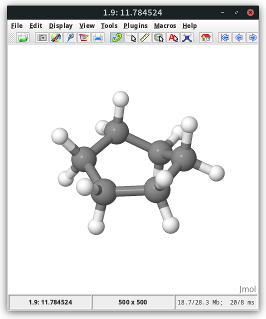
The final reaction path can be found in stringfile.xyz0000 and can be visualized with the molecule viewer of your choice.
Note that the comment line contains the energy difference to the reactant in kcal/mol and some viewers, like molden, can plot this while visualizing the path.
In jmol the energy is visible in the lower left corner
To visualize the path extract the relative energies from the comment lines with
❯ awk '$1 ~ /-?[0-9]+\.[0-9]+/ {print $0}' stringfile.xyz0000 > path000.txt
You can view the energy profile with xmgrace.
Exercise
Compute the inversion barrier with GFN2-xTB and plot the energy profile.
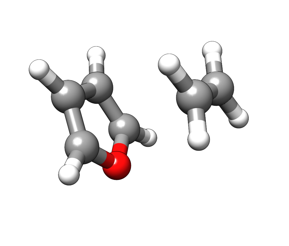
Diels-Alder reaction#
For the next example we will investigate a reaction path for a Diels-Alder reaction, including bond breaking / formation in the path search. This time we want to investigate the effect of different methods for the final barrier height. In the input file we choose more nodes and set the bond breaking flag.
# FSM/GSM/SSM inpfileq
------------ String Info --------------------------------
SM_TYPE                 GSM    # SSM, FSM or GSM
RESTART                 0      # read restart.xyz
MAX_OPT_ITERS           80     # maximum iterations
STEP_OPT_ITERS          30     # for FSM/SSM
CONV_TOL                0.0005 # perp grad
ADD_NODE_TOL            0.1    # for GSM
SCALING                 1.0    # for opt steps
SSM_DQMAX               0.8    # add step size
GROWTH_DIRECTION        0      # normal/react/prod: 0/1/2
INT_THRESH              2.0    # intermediate detection
MIN_SPACING             5.0    # node spacing SSM
BOND_FRAGMENTS          1      # make IC's for fragments
INITIAL_OPT             0      # opt steps first node
FINAL_OPT               150    # opt steps last SSM node
PRODUCT_LIMIT           100.0  # kcal/mol
TS_FINAL_TYPE           1      # any/delta bond: 0/1
NNODES                  20     # including endpoints
---------------------------------------------------------
For the cycloaddition we use a furan and ethene molecule
15

C   -1.05403119  -0.85921125  -1.07844148
O   -0.74716995  -1.59204846   0.00037929
C    1.91999122   0.31825506  -0.65929558
C   -1.56348463   0.34378897  -0.70923752
C   -1.05432765  -0.85883374   1.07895685
C    1.92016161   0.31774885   0.65905212
C   -1.56373749   0.34366980   0.70888173
H   -0.86626022  -1.30691107  -2.03849048
H    2.21980037  -0.54462844  -1.23619995
H    1.61547946   1.18008308  -1.23636699
H   -1.89753571   1.13638114  -1.35561033
H   -0.86679445  -1.30614725   2.03907198
H    2.21960266  -0.54586684   1.23524723
H    1.61610877   1.17913244   1.23678680
H   -1.89780281   1.13623322   1.35526633
15

C   -0.33650300  -0.52567500  -1.05221900
O   -0.49920800  -1.44888700   0.00032300
C    1.08232400   0.03657400  -0.76729600
C   -1.29917500   0.57935400  -0.66347200
C   -0.33671300  -0.52527900   1.05252700
C    1.08262000   0.03575900   0.76715400
C   -1.29967800   0.57933100   0.66328300
H   -0.47204500  -0.99959700  -2.02194900
H    1.84062900  -0.63339500  -1.16910900
H    1.22478200   1.02637400  -1.19722100
H   -1.79017300   1.24152200  -1.35666900
H   -0.47213100  -0.99881000   2.02246200
H    1.84129300  -0.63425300   1.16825900
H    1.22479600   1.02528600   1.19777000
H   -1.79081700   1.24169700   1.35615700
For this path we want to investigate GFN1-xTB, GFN2-xTB, DFTB3-D4, DFTB2-D4, and LC-DFTB2-D4. To ease the reaction path search the reactants should be optimized before running the path search.
Geometry = xyzFormat {
<<< "struc.xyz"
}

Hamiltonian = xTB {
  Method = "GFN2-xTB"
}

Options = {
  WriteAutotestTag = Yes
  WriteDetailedOut = No
}
Analysis { CalculateForces = Yes }
ParserOptions = { ParserVersion = 10 }
Parallel = { UseOmpThreads = Yes }
Geometry = xyzFormat {
<<< "struc.xyz"
}

Hamiltonian = xTB {
  Method = "GFN1-xTB"
}

Options = {
  WriteAutotestTag = Yes
  WriteDetailedOut = No
}
Analysis { CalculateForces = Yes }
ParserOptions = { ParserVersion = 10 }
Parallel = { UseOmpThreads = Yes }
Geometry = xyzFormat {
<<< "struc.xyz"
}

Hamiltonian = DFTB {
  SCC = Yes
  MaxAngularMomentum {
    H = "s"
    C = "p"
    O = "p"
  }
  HubbardDerivs {
    H = -0.1857
    C = -0.1492
    O = -0.1575
  }
  ThirdOrderFull = Yes
  HCorrection = Damping { Exponent = 4.0 }
  SlaterKosterFiles = Type2FileNames {
    Prefix = "slakos/origin/3ob-3-1/"
    Separator = "-"
    Suffix = ".skf"
  }
  Dispersion = DFTD4 {
    s6 = 1.0
    s9 = 0.0
    s8 = 0.4727337
    a1 = 0.5467502
    a2 = 4.4955068
  }
}

Options = {
  WriteAutotestTag = Yes
  WriteDetailedOut = No
}
Analysis { CalculateForces = Yes }
ParserOptions = { ParserVersion = 10 }
Parallel = { UseOmpThreads = Yes }
Geometry = xyzFormat {
<<< "struc.xyz"
}

Hamiltonian = DFTB {
  SCC = Yes
  MaxAngularMomentum {
    H = "s"
    C = "p"
    O = "p"
  }
  SlaterKosterFiles = Type2FileNames {
    Prefix = "slakos/origin/mio-1-1/"
    Separator = "-"
    Suffix = ".skf"
  }
  Dispersion = DFTD4 {
    s6 = 1.0
    s9 = 0.0
    s8 = 1.1948145
    a1 = 0.6074567
    a2 = 4.9336133
  }
}

Options = {
  WriteAutotestTag = Yes
  WriteDetailedOut = No
}
Analysis { CalculateForces = Yes }
ParserOptions = { ParserVersion = 10 }
Parallel = { UseOmpThreads = Yes }
Geometry = xyzFormat {
<<< "struc.xyz"
}

Hamiltonian = DFTB {
  SCC = Yes
  MaxAngularMomentum {
    H = "s"
    C = "p"
    O = "p"
  }
  RangeSeparated = LC { Screening = NeighbourBased {} }
  SlaterKosterFiles = Type2FileNames {
    Prefix = "slakos/origin/ob2-1-1/shift/"
    Separator = "-"
    Suffix = ".skf"
  }
  Dispersion = DFTD4 {
    s6 = 1.0
    s9 = 0.0
    s8 = 2.7611320
    a1 = 0.6037249
    a2 = 5.3900004
  }
}

Options = {
  WriteAutotestTag = Yes
  WriteDetailedOut = No
}
Analysis { CalculateForces = Yes }
ParserOptions = { ParserVersion = 10 }
Parallel = { UseOmpThreads = Yes }
For each of the five models we create a separate calculation directory and add the required dftb_in.hsd as well as the reactant and product input structure.
To optimize both structures we perform a short optimization with the reactant and product.
An example for running the optimization is given below
❯ for i in reactant product; do
mkdir -p preopt-$i
cp $i.xyz preopt-$i/struc.xyz
cp dftb_in.hsd preopt-$i/dftb_in.hsd
echo "Driver = GeometryOptimization {}" >> preopt-$i/dftb_in.hsd
pushd preopt-$i
dftb+ | tee dftb.out
popd
done
From the preoptimized structures we again setup a reaction path for the GSM program. The following directory structure should be present before starting the actual reaction path search.
❯ ln -s $(which ograd)
❯ mkdir scratch
❯ cat preopt-reactant/geo_end.xyz preopt-product/geo_end.xyz > scratch/initial0000.xyz
❯ tree .
.
├── dftb_in.hsd
├── inpfileq
├── ograd -> /path/to/ograd
├── preopt-product
│   └── ...
├── preopt-reactant
│   └── ...
├── product.xyz
├── reactant.xyz
└── scratch
    └── initial0000.xyz
Exercise
Compare the barrier heights obtained with the different methods. Does any of the tested methods provide significant different results? Is the relative difference of the barrier heights in this case as expected?
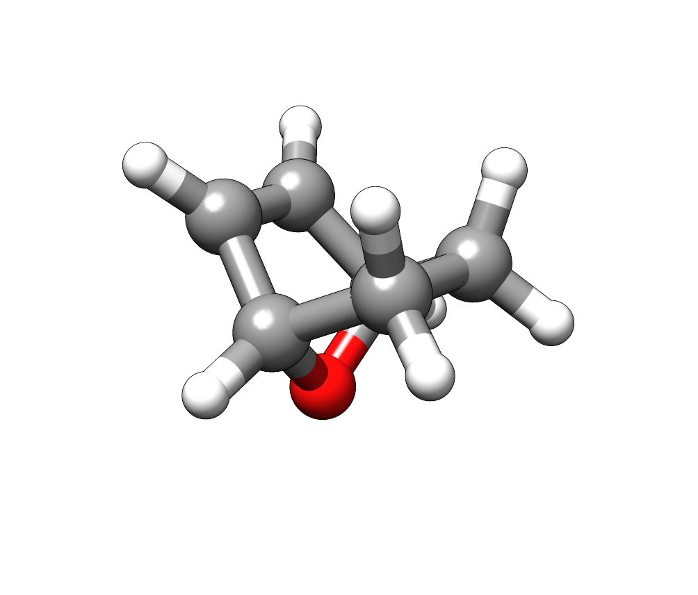
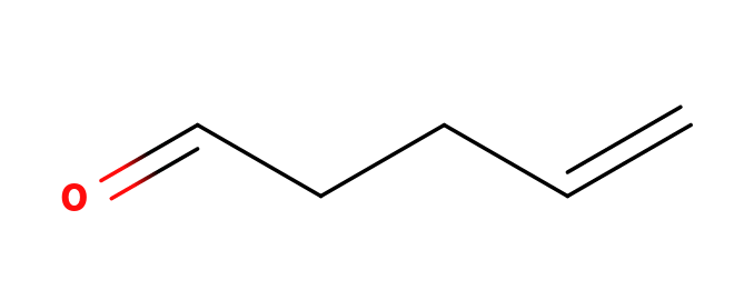
Claisen rearrangement reaction#
Another example is the Claisen rearrangement. As starting structure we use allyl vinyl ether and the corresponding pentenale.
14

C       0.33830681      -0.40028145       0.06863012
C       0.10595161      -0.26718767       1.36421188
H       1.33077226      -0.61906183      -0.27493881
H      -0.42216146      -0.28728678      -0.68244497
O      -1.06599246      -0.01419187       2.00107453
H       0.89080386      -0.36692363       2.10223944
C      -2.24339525       0.08535540       1.21865884
H      -3.06296651       0.00347496       1.94095352
C      -2.38810216       1.37002374       0.45318426
H      -2.30704191      -0.76808842       0.53050462
H      -3.21531691       1.36845744      -0.24273208
C      -1.61866094       2.43160218       0.59926563
H      -0.79697159       2.43969569       1.29630648
H      -1.77723230       3.33005423       0.02997950

14

C       0.05083404       0.47756955       0.03067754
C       0.22099793      -0.53384083       1.12248949
H       1.00063556       0.99546491      -0.11008883
H      -0.23550427      -0.01507412      -0.90051555
O      -0.06214314      -1.70052772       1.01406801
H       0.61484477      -0.11647527       2.06863484
C      -3.09105601       0.69502179       1.56213016
H      -4.07672239       0.25168355       1.53446340
C      -2.38605593       0.89986170       0.46164886
H      -2.72406577       0.97143579       2.54163695
H      -2.77578741       0.61350077      -0.51143129
C      -1.01585926       1.51412664       0.44531292
H      -0.76139644       1.92312285       1.42742393
H      -0.99072867       2.32977240      -0.28155745
Exercise
Compute the barrier height for the Claisen rearrangement. The expected barrier with GFN2-xTB is around 40 kcal/mol.
Tip
The provided input structure might not be optimal, try to prepare the structures to find the optimal reaction path.
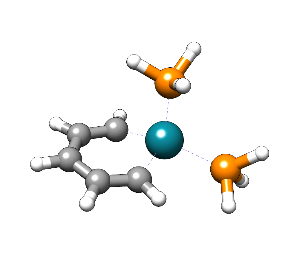
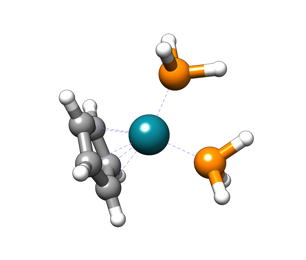
Transition metal reactions#
Another interesting application of the GSM path finder together with tight binding methods is the investigation of transition metal complexes.2 For this exercises we will investigate several different reactions using the xTB Hamiltonian.
Metallabenzene vs. Rhodium Cp complex
19

C           -0.57502200000000       -1.29836600000000        0.75007100000000
C           -1.92930100000000       -1.34370800000000        1.08475100000000
C           -2.94722600000000       -0.63129900000000        0.42296400000000
C           -2.70781300000000        0.19779700000000       -0.69430700000000
C           -1.42207200000000        0.39056700000000       -1.18041300000000
Rh           0.31309200000000        0.02021600000000       -0.38482800000000
P            0.49101000000000        1.97255500000000        0.73434700000000
P            2.42912400000000       -0.98184200000000       -0.02285400000000
H            0.08895600000000       -1.89538300000000        1.40253400000000
H           -2.23621800000000       -2.01113400000000        1.90415900000000
H           -3.98331200000000       -0.77766100000000        0.75472100000000
H           -1.31162700000000        0.89114000000000       -2.16741100000000
H           -3.57836500000000        0.59994000000000       -1.23258900000000
H            3.11656700000000       -1.46461400000000       -1.17511700000000
H            2.46754600000000       -2.20072400000000        0.71804700000000
H            3.59504100000000       -0.41813400000000        0.58900900000000
H            1.29853500000000        3.13588500000000        0.50288200000000
H            0.86763700000000        1.80867300000000        2.09579800000000
H           -0.72730400000000        2.67165900000000        0.95444800000000
19

C           -1.52397380000000       -1.77134579000000        0.13991595000000
C           -2.10229449000000       -0.93083677000000        1.14371125000000
C           -2.37007063000000        0.32503169000000        0.51167613000000
C           -2.10083390000000        0.20618203000000       -0.91457606000000
C           -1.57950456000000       -1.08577775000000       -1.14369436000000
Rh          -0.16948171000000       -0.00343404000000        0.31231974000000
P            0.67247773000000        1.97112569000000        0.84740684000000
P            1.84120403000000       -0.92575934000000        0.33533038000000
H           -1.19640273000000       -2.80295205000000        0.28642744000000
H           -2.26609676000000       -1.18272179000000        2.19134946000000
H           -2.81145758000000        1.19884516000000        0.99603525000000
H           -1.26680946000000       -1.50034294000000       -2.10296656000000
H           -2.26852428000000        0.98204390000000       -1.66275319000000
H            2.37748820000000       -1.58164181000000       -0.81947971000000
H            2.16348741000000       -1.98758278000000        1.24088608000000
H            2.98962124000000       -0.12596819000000        0.61348773000000
H            2.08150513000000        2.12495151000000        1.01136094000000
H            0.29753994000000        2.63754823000000        2.05846777000000
H            0.48137422000000        3.11820203000000        0.01130690000000
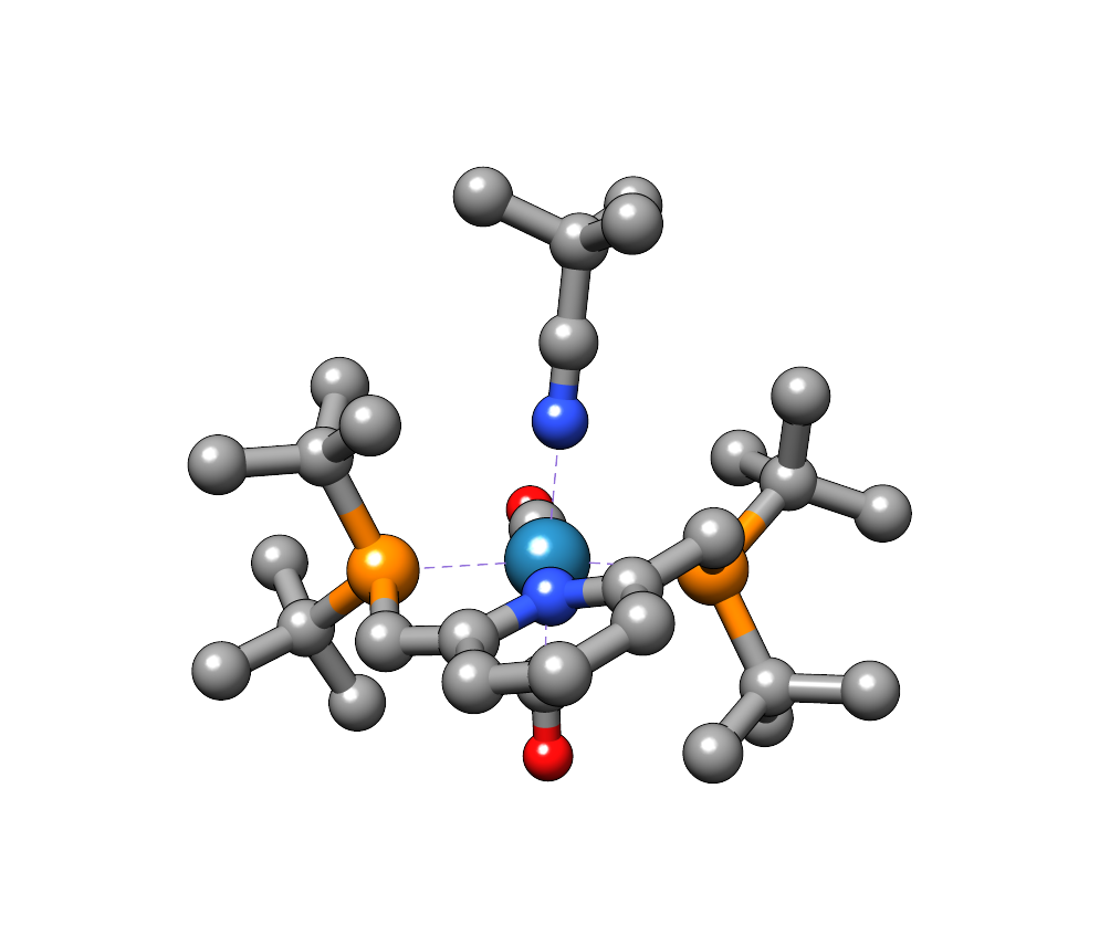
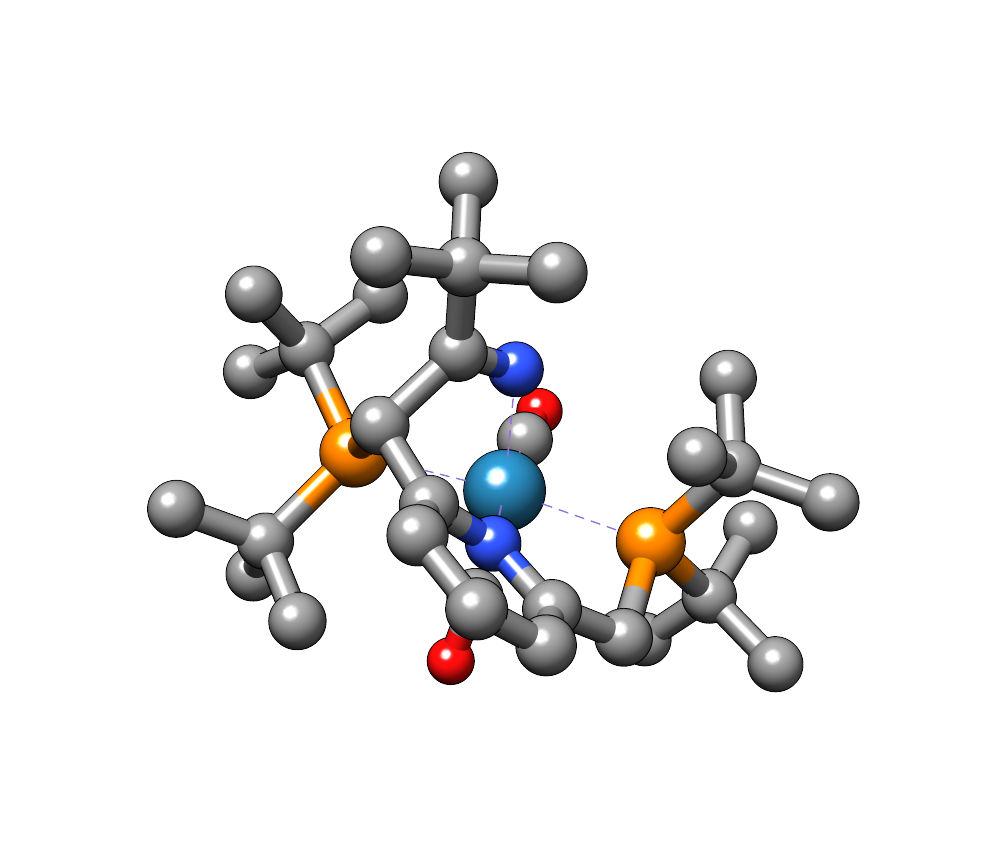
Rhenium PNP pincer complex
88

C            1.12571700000000       -0.64396800000000        2.39383100000000
C            1.23314900000000       -1.07706400000000        3.71158300000000
C            0.11093500000000       -1.72174600000000        4.29650200000000
C           -1.04928000000000       -1.87466900000000        3.57130100000000
C           -1.15740100000000       -1.37679100000000        2.22231300000000
N           -0.01024800000000       -0.79496000000000        1.65214300000000
H            0.16889100000000       -2.09443400000000        5.32552600000000
H            2.16508300000000       -0.93280200000000        4.26417700000000
H           -1.92595000000000       -2.36258200000000        4.00777600000000
C           -2.35433100000000       -1.43785500000000        1.49736100000000
H           -3.24153400000000       -1.82671200000000        2.00870000000000
C            2.29448900000000        0.03394500000000        1.71184800000000
H            3.23370900000000       -0.15327300000000        2.25939300000000
H            2.11907300000000        1.12355700000000        1.71013900000000
P           -2.47443800000000       -0.47747800000000        0.00963300000000
P            2.36563000000000       -0.46009200000000       -0.09474200000000
C           -0.21473000000000        0.09655100000000       -2.39083300000000
O           -0.34324300000000        0.37706500000000       -3.52654900000000
C            0.24919500000000        2.86506200000000        0.13420900000000
C           -3.31254600000000        1.19148700000000        0.53505400000000
C           -4.79886000000000        1.07332400000000        0.91840500000000
C           -2.55714500000000        1.62357100000000        1.81209700000000
C           -3.14817500000000        2.24375900000000       -0.57871900000000
H           -5.44725000000000        0.86715500000000        0.05157800000000
H           -4.95750200000000        0.28769200000000        1.67721300000000
H           -5.13326900000000        2.03315400000000        1.35861600000000
H           -1.46483100000000        1.58166300000000        1.69121500000000
H           -2.84907300000000        2.65902400000000        2.07529800000000
H           -2.81772300000000        0.96636200000000        2.65694800000000
H           -3.42692800000000        3.24237500000000       -0.19125700000000
H           -2.11241000000000        2.28348000000000       -0.94939600000000
H           -3.80052500000000        2.03326400000000       -1.43909100000000
C           -3.70118000000000       -1.37762500000000       -1.16013400000000
C           -4.19161800000000       -0.43051400000000       -2.27181800000000
C           -2.96949500000000       -2.55192500000000       -1.83044200000000
C           -4.88931700000000       -1.97399200000000       -0.37587000000000
H           -4.86862400000000        0.35218800000000       -1.89388800000000
H           -3.34434700000000        0.05148000000000       -2.78979200000000
H           -4.75395500000000       -1.01872500000000       -3.02113300000000
H           -2.54238300000000       -3.23981100000000       -1.08480900000000
H           -3.69812400000000       -3.11667500000000       -2.44258900000000
H           -2.16574500000000       -2.20254200000000       -2.49642500000000
H           -5.55142600000000       -2.50439500000000       -1.08638300000000
H           -4.53529900000000       -2.71038600000000        0.36467600000000
H           -5.49422200000000       -1.21811000000000        0.14371500000000
C            3.55061500000000        0.82161100000000       -0.95197200000000
C            2.88386400000000        1.18773800000000       -2.29390700000000
C            3.66393000000000        2.08516100000000       -0.07779100000000
C            4.98838600000000        0.34530900000000       -1.23297600000000
H            2.73636900000000        0.30003000000000       -2.93152500000000
H            1.89598900000000        1.64772800000000       -2.13875200000000
H            3.52796200000000        1.90380400000000       -2.83871500000000
H            4.19999500000000        1.88865700000000        0.86598600000000
H            4.23336100000000        2.85377400000000       -0.63396900000000
H            2.67695000000000        2.50338800000000        0.16232300000000
H            5.50496700000000        1.14284000000000       -1.79969200000000
H            5.55883800000000        0.17661300000000       -0.30694900000000
H            5.02415700000000       -0.56777300000000       -1.84670900000000
C            3.19424400000000       -2.18778100000000       -0.02973800000000
C            2.32476900000000       -3.08050500000000        0.88957300000000
C            3.22411600000000       -2.75884900000000       -1.46269900000000
C            4.61483700000000       -2.20094900000000        0.57940600000000
H            2.49358000000000       -2.83779400000000        1.95089600000000
H            1.24875400000000       -2.99543800000000        0.69405900000000
H            2.62027300000000       -4.13321500000000        0.72640100000000
H            3.84428900000000       -2.14541200000000       -2.13803300000000
H            3.65998000000000       -3.77500600000000       -1.43828500000000
H            2.21530600000000       -2.83479000000000       -1.89243100000000
H            4.85926500000000       -3.24310100000000        0.85581500000000
H            5.38911100000000       -1.85936100000000       -0.11941500000000
H            4.67844500000000       -1.59775500000000        1.50215500000000
C           -0.10073700000000       -2.20376900000000       -1.01896800000000
O           -0.05683900000000       -3.32630100000000       -1.36209900000000
Re          -0.06366100000000       -0.34534900000000       -0.52165300000000
N            0.12443900000000        1.71628400000000       -0.06484500000000
C            0.40317500000000        4.30831600000000        0.40017200000000
C            1.14159700000000        4.47520100000000        1.75397800000000
C            1.21692000000000        4.94754800000000       -0.75483900000000
C           -0.99550800000000        4.97061000000000        0.48067600000000
H            0.57118500000000        4.00405800000000        2.57133100000000
H            2.14658900000000        4.02398200000000        1.72004200000000
H            1.24924800000000        5.55119000000000        1.97365500000000
H            0.70084100000000        4.81011000000000       -1.71926100000000
H            1.32052200000000        6.02923800000000       -0.56257500000000
H            2.22286200000000        4.50602800000000       -0.82940400000000
H           -0.86489400000000        6.04481400000000        0.69763300000000
H           -1.53741500000000        4.86649700000000       -0.47219800000000
H           -1.60184600000000        4.51814500000000        1.28050400000000
88

C            0.86149444000000       -1.78771344000000        1.64010558000000
C            0.75488202000000       -2.21922912000000        2.96638390000000
C           -0.22095966000000       -1.64978763000000        3.80253364000000
C           -1.05455545000000       -0.64866456000000        3.30189976000000
C           -0.92867634000000       -0.25759739000000        1.95687359000000
N            0.00130184000000       -0.84953088000000        1.14602570000000
H           -0.31414785000000       -1.97799915000000        4.84272958000000
H            1.44287095000000       -2.98102981000000        3.34316028000000
H           -1.80701362000000       -0.16828577000000        3.93365044000000
C           -1.66626744000000        0.89602488000000        1.34818749000000
H           -2.50254236000000        1.21211295000000        1.98744432000000
C            1.94789664000000       -2.27044797000000        0.70920263000000
H            1.55101500000000       -3.07014117000000        0.05469893000000
H            2.79346968000000       -2.68778637000000        1.28236901000000
P           -2.13609273000000        0.47893014000000       -0.45596110000000
P            2.41839474000000       -0.89567018000000       -0.50053969000000
C            0.49793183000000        0.66903180000000       -2.64300347000000
O            0.74846690000000        1.13406599000000       -3.69421715000000
C           -0.51934595000000        1.97628318000000        1.14252530000000
C           -2.91815774000000        2.08694289000000       -1.17964384000000
C           -3.64734969000000        2.89430282000000       -0.08970012000000
C           -1.79493535000000        2.94550044000000       -1.80368738000000
C           -3.89663669000000        1.75784093000000       -2.32610709000000
H           -4.43933710000000        2.31582449000000        0.41177557000000
H           -2.94389839000000        3.25484094000000        0.67495465000000
H           -4.11849809000000        3.78202847000000       -0.55190962000000
H           -1.37598705000000        2.45379423000000       -2.69449384000000
H           -2.23585873000000        3.91020324000000       -2.11870890000000
H           -0.96735981000000        3.14065205000000       -1.10956152000000
H           -4.19712746000000        2.71130095000000       -2.79853091000000
H           -3.41604669000000        1.14002839000000       -3.10283668000000
H           -4.81469005000000        1.25550791000000       -1.98377167000000
C           -3.48995181000000       -0.87303837000000       -0.31854511000000
C           -3.79796745000000       -1.44508072000000       -1.72180843000000
C           -2.93886858000000       -2.03904410000000        0.53388402000000
C           -4.77671142000000       -0.35961522000000        0.35729730000000
H           -4.28641726000000       -0.71900713000000       -2.38473099000000
H           -2.88349932000000       -1.81392757000000       -2.21041988000000
H           -4.48484815000000       -2.30392753000000       -1.60251513000000
H           -2.84659891000000       -1.76989151000000        1.59707203000000
H           -3.65224036000000       -2.88067274000000        0.46159422000000
H           -1.96231420000000       -2.39128464000000        0.17006063000000
H           -5.47404456000000       -1.20797269000000        0.49089836000000
H           -4.57144771000000        0.06162204000000        1.35726321000000
H           -5.29765645000000        0.40348968000000       -0.24200125000000
C            3.59944579000000        0.25164222000000        0.47607065000000
C            3.58718371000000        1.61636935000000       -0.25012236000000
C            2.96830771000000        0.43988887000000        1.86924432000000
C            5.03872775000000       -0.25474999000000        0.67563828000000
H            4.00379416000000        1.55323068000000       -1.26791119000000
H            2.55402709000000        2.00319380000000       -0.30329275000000
H            4.20614663000000        2.33155552000000        0.32495740000000
H            3.04100438000000       -0.47246148000000        2.48504790000000
H            3.51117714000000        1.24461479000000        2.39827932000000
H            1.91439376000000        0.74142145000000        1.78705832000000
H            5.57584579000000        0.47099678000000        1.31524502000000
H            5.06685716000000       -1.23073383000000        1.19140386000000
H            5.60080441000000       -0.33775522000000       -0.26783006000000
C            3.41489389000000       -1.80539212000000       -1.85917774000000
C            2.43574530000000       -2.55734763000000       -2.78065322000000
C            4.14151619000000       -0.74748112000000       -2.71677803000000
C            4.40792441000000       -2.83769874000000       -1.28526836000000
H            1.84786755000000       -3.31835121000000       -2.24287101000000
H            1.73548180000000       -1.86756021000000       -3.27466575000000
H            3.02536524000000       -3.07681208000000       -3.55933894000000
H            4.94358605000000       -0.23065258000000       -2.16684333000000
H            4.60278475000000       -1.25058200000000       -3.58673381000000
H            3.43292104000000        0.00674948000000       -3.09926855000000
H            4.94367264000000       -3.31779637000000       -2.12551231000000
H            5.16103559000000       -2.39468254000000       -0.61976444000000
H            3.88251072000000       -3.63745425000000       -0.73543224000000
C           -0.29510138000000       -1.80538246000000       -1.69345890000000
O           -0.68503822000000       -2.85215138000000       -2.08230874000000
Re           0.17059664000000       -0.11132819000000       -0.90929276000000
N            0.34045026000000        1.74507402000000        0.23439942000000
C           -0.41939020000000        3.18886841000000        2.11875167000000
C            0.90848217000000        3.06052644000000        2.89879991000000
C           -0.36629646000000        4.48904036000000        1.28622862000000
C           -1.57166982000000        3.26588979000000        3.13880383000000
H            0.93465436000000        2.12833861000000        3.49024003000000
H            1.75604884000000        3.05043816000000        2.19658630000000
H            1.02823907000000        3.91378980000000        3.59174581000000
H           -1.32186630000000        4.68260456000000        0.76990072000000
H           -0.15028200000000        5.35364666000000        1.94008388000000
H            0.42698569000000        4.40715826000000        0.52524233000000
H           -1.43238026000000        4.14829339000000        3.78862083000000
H           -2.55839372000000        3.36655257000000        2.65439611000000
H           -1.59615894000000        2.37606467000000        3.79246860000000
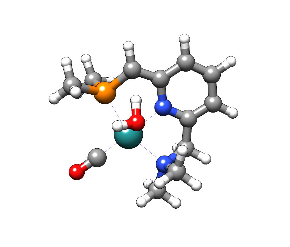
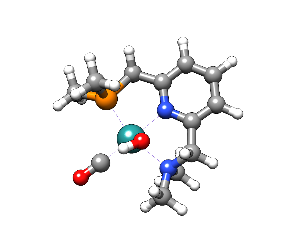
Ruthenium pincer complex
39

C            2.14156830195641       -1.29348060521416       -0.95757067905303
C            2.24700760711555        0.14233347609941       -0.50586093650040
N            1.04338872702218        0.68595310415767       -0.22185519901871
C            0.89757296527426        2.00324864849573        0.19432967469119
C            2.09375233592471        2.78900864784732        0.28220632952698
C            3.32492176488136        2.22699525794963       -0.01469668283423
C            3.42986421449946        0.87038576546755       -0.41268411738744
C           -0.41468565587209        2.42184591804414        0.53889610156852
P           -1.72895705533737        1.36989135386445       -0.08676456007610
H            4.39410438883000        0.41090473720723       -0.64414007610268
H            2.01554759488035        3.83423341442195        0.59443444806665
H            4.23044786169423        2.83957470692107        0.06107428757122
C            0.77151950517073       -3.30565077713550       -0.81971604154894
C            1.62520412919640       -2.28352760047943        1.21254788356364
H           -0.58620193520706        3.47916027797597        0.77793436121436
H            3.11828334116379       -1.81373057062002       -0.90082176198738
H            1.79253913157996       -1.31229332047328       -2.00470932781361
C           -2.37448438095365        2.03978448537501       -1.68896016087244
C           -3.17725535922990        1.64701934153411        1.02959756453653
H           -3.20040386198274        1.40394670099854       -2.05196954383466
H           -2.72571782167635        3.08009680871532       -1.57067572427195
H           -1.55242767030124        2.00864301819123       -2.42160586033589
H           -4.04100880702443        1.06397521687219        0.66870638844135
H           -2.92580808692839        1.31399209358725        2.05001475980488
H           -3.44703280439002        2.71753432492179        1.06366288079101
H            2.52711447353895       -2.92872046225583        1.17221107603511
H            1.87157642421579       -1.32632983838760        1.69366410813994
H            0.84081610841256       -2.78264715239870        1.80103975628715
H            1.67094180241586       -3.94887822037930       -0.91756154340895
H            0.01177103493782       -3.82890951607527       -0.22062069509309
H            0.35360313945659       -3.08938725264281       -1.81348348684775
C           -2.08990509620891       -1.70656155341050        0.00098802708439
O           -3.05088180975026       -2.38495566492066        0.02691652376577
Ru          -0.60689736425803       -0.60601946718620       -0.09131251822389
H           -0.72348988353592       -0.75718225033382       -1.67431224162697
O           -0.19928336645442       -0.04572652320111        2.16623659808879
H           -1.02943439234246       -0.20830869311707        2.64988349495872
H           -0.22935269685405        0.94192520512638        1.95999630422654
N            1.10760319614222       -2.02587303554773       -0.15370941152654
39

C            2.22934206000000       -1.26375759000000        0.68371909000000
C            2.28158720000000        0.17526736000000        0.24446482000000
N            1.07751903000000        0.68845263000000       -0.11138669000000
C            0.92766202000000        2.00760156000000       -0.39400028000000
C            2.03095097000000        2.87112410000000       -0.32952961000000
C            3.29042609000000        2.35206951000000        0.00062251000000
C            3.42155580000000        0.98597375000000        0.28562791000000
C           -0.46179965000000        2.43581733000000       -0.79321757000000
P           -1.72276986000000        1.20829520000000       -0.11988634000000
H            4.38916475000000        0.55422979000000        0.55754772000000
H            1.90090963000000        3.93478693000000       -0.54860748000000
H            4.16423220000000        3.01037348000000        0.03926767000000
C            1.72162376000000       -2.32599418000000       -1.46706228000000
C            0.89515918000000       -3.28121792000000        0.62809508000000
H           -0.55298064000000        2.35667091000000       -1.89411302000000
H            1.82326294000000       -1.25460762000000        1.71485737000000
H            3.22678123000000       -1.74481329000000        0.65077788000000
C           -3.19417300000000        1.49854417000000       -1.18870498000000
C           -2.21535271000000        1.92624960000000        1.50994332000000
H           -4.01488282000000        0.85462369000000       -0.83033218000000
H           -3.52108836000000        2.55308519000000       -1.16892242000000
H           -2.94183227000000        1.19603757000000       -2.21784989000000
H           -3.08067893000000        1.35789888000000        1.89223815000000
H           -1.37026601000000        1.76188687000000        2.19905160000000
H           -2.47811893000000        2.99699945000000        1.44678261000000
H            1.80132425000000       -3.90283762000000        0.78450306000000
H            0.46084788000000       -2.97040985000000        1.59137142000000
H            0.15511648000000       -3.85113240000000        0.04676705000000
H            2.62583777000000       -2.96997336000000       -1.42745344000000
H            0.92624614000000       -2.82866640000000       -2.03557756000000
H            1.96286250000000       -1.37761512000000       -1.97011177000000
C           -1.96679093000000       -1.81207395000000       -0.21667655000000
O           -2.90250672000000       -2.51561928000000       -0.31712478000000
Ru          -0.52761306000000       -0.66165773000000       -0.10993849000000
H           -0.54751212000000       -0.60916247000000       -1.75694704000000
O           -0.14464432000000       -0.69054709000000        1.99512044000000
H           -0.95297155000000       -0.99660875000000        2.44148419000000
H           -0.66328457000000        3.48492011000000       -0.51170604000000
N            1.22496156000000       -2.03695347000000       -0.10513049000000
Exercise
Find the reaction paths for the three transition metal reactions with GFN2-xTB. Compare the computed barrier heights and reaction energies with the reference values computed by localized coupled cluster or double hybrid density functionals given below (in kcal/mol).
Metal |
Barrier |
Reaction |
|---|---|---|
Ru |
20.27 |
–56.96 |
Re |
2.66 |
–9.35 |
Rh |
10.35 |
–3.32 |
Summary#
You learned…
to prepare starting structures for a reaction path search
perform a reaction path search with the growing string methods
compare reaction paths from different semiempirical methods
Literature#
- 1
Paul M Zimmerman. Growing string method with interpolation and optimization in internal coordinates: method and examples. J. Chem. Phys., 138(18):184102, 2013. doi:10.1063/1.4804162.
- 2
Sebastian Dohm, Markus Bursch, Andreas Hansen, and Stefan Grimme. Semiautomated transition state localization for organometallic complexes with semiempirical quantum chemical methods. J. Chem. Theory Comput., 16(3):2002–2012, 2020. doi:10.1021/acs.jctc.9b01266.